Examples
Included with the QOCCM GitHub repository are some example files that will be used to run these QOCCM examples. You’ll need to download these files from the QOCCM GitHub repository if you installed QOCCM via pip.
Simple Example: Idealized Experiments
In this example we will show you how to generate idealized experiments. This example is forced with atmospheric CO2 consistent with an unmitigated climate change scenario (RCP8.5). By selecting a mixed layer depth of 51 meters, QOCCM in this example will match the carbon uptake of the Community Earth Sysetm Model (CESM) ocean component model.
Start in the qoccm directory you cloned from GitHub or copy the files ATM_CO2.nc and GMSSTA.nc from the qoccm directory to you working directory.
The first step is to specify the model timestep and ocean mixed layer depth. Smaller timesteps (<0.5 years) combined with shallow mixed layer depths (<90m) currently cause numerical instability.
import qoccm
import xarray as xr
import numpy as np


OceanMLDepth = 51 # this gives the best fit to the CESM

year_i = 1850.5
year_f = 2080.5
nsteps = 230

time_step = (year_f-year_i)/nsteps
Note that year_i must be the start of the industrial revolution, which is 1850 in this example. QOCCM is always intialized from a preindustrial state, because one of the basic assumptions of the model is that \(C_{ant}(t_i) = 0\).
Next load in the forcings: global mean sea surface temperature anomaly (\(Kelvin\); DT), and atmospheric CO2 (\(ppm\); atm_co2):
atmos_co2 = xr.open_dataarray(f'ATM_CO2.nc')
DT = xr.open_dataarray('GMSSTA.nc')
DT is this example is diagnosed from the ocean component model of the CESM-LENS (Kay et al. 2015).
In this next step, we interpolate the forcings to the points in time for the given timestep. The forcings must have dimensions ‘year’, which QOCCM will use to infer the timestep.
atmos_co2 = atmos_co2.interp(year=np.linspace(year_i,year_f,nsteps))
DT = DT.interp(year=np.linspace(year_i,year_f,nsteps))
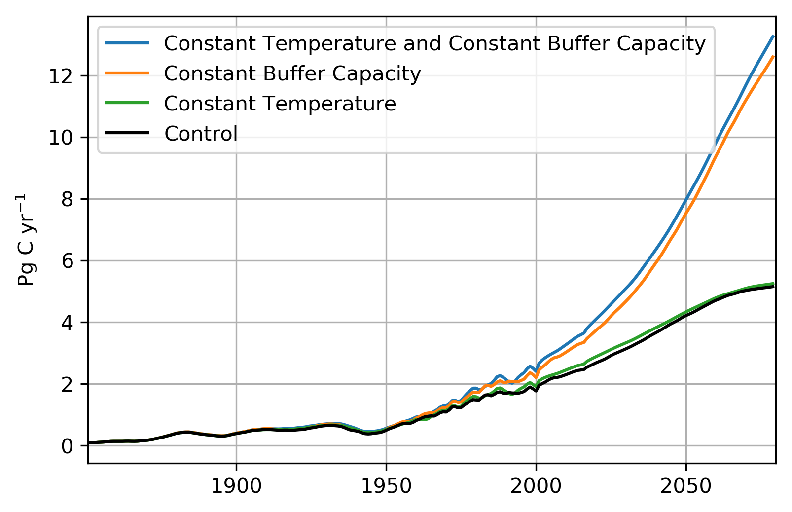
Run model and plot the results:
import matplotlib.pyplot as plt

plt.figure(dpi=300)

# linear buffering and constant solubility
ds = qoccm.ocean_flux(atmos_co2,
                      OceanMLDepth=OceanMLDepth, HILDA=True,
                      DT=None,
                      temperature='constant', chemistry='constant',
                     )
flux = ds.F_as
plt.plot(flux.year,flux,label = 'Constant Temperature and Constant Buffer Capacity')

# linear buffering
ds = qoccm.ocean_flux(atmos_co2,
                      OceanMLDepth=OceanMLDepth, HILDA=True,
                      DT=DT,
                      temperature='variable', chemistry='constant',
                     )
flux = ds.F_as
plt.plot(flux.year,flux,label='Constant Buffer Capacity')

# constant solubility
ds = qoccm.ocean_flux(atmos_co2,
                      OceanMLDepth=OceanMLDepth, HILDA=True,
                      DT=None,
                      temperature='constant', chemistry='variable',
                     )
flux = ds.F_as
plt.plot(flux.year,flux,label = 'Constant Temperature',color='tab:green')

# control
ds = qoccm.ocean_flux(atmos_co2,
                      OceanMLDepth=OceanMLDepth, HILDA=True,
                      DT=DT,
                      temperature='variable', chemistry='variable',
                     )
flux = ds.F_as
plt.plot(flux.year,flux,label='Control',color='k')
plt.ylabel('Pg C yr$^{-1}$')
plt.grid()
plt.xlim(1850.5,2080)
plt.legend()
Output: