Methodology
Model Dynamics
QOCCM is based on the model of Joos et al. (1996). QOCCM is in the same class of models that generate the CO2 concentration scenarios that are used to force the Earth System Models of CMIP6. For a detailed description of the model see Ridge and McKinley (2020) and Joos et al. (1996). The model consists of two equations that are solved at each timestep:
The mixed layer concentration of anthropogenic carbon, \(C_{ant}(t)\), is calculated as the convultion integral of the air-sea \(C_{ant}\) flux, \(F_{ant}(t)\), and mixed layer impulse response function, \(r(t)\). The mixed layer impulse response function characterizes the time that a unit pulse would take to leave the surface ocean mixed layer, and can be calculated for any ocean carbon cycle model. Included in this package is r(t) for two models, the HILDA model (a box diffusion model) and a three-dimensional Ocean General Ciculation Model (OGCM; Sarmiento et al., 1992).
Effective ocean mixed layer depth, the depth of the ocean that actually exchanges with the atmosphere, is \(h\). This is used as a tuning parameter when fitting QOCCM to Earth System Models. The air-sea flux is calculated as the difference between surface ocean partial pressure of CO2 (\(pCO_{2}^{ocn}\)) and atmosphere CO2 (\(pCO_{2}^{atm}\)), times a gas exchange coefficient, \(k_g\) (\(m^{-2}~year^{-1}\)). A conversion factor, c, converts the flux from \(ppm~m^{-2}~year^{-1}\) into units of \(\mu mol~kg^{-1} m^{-2}~year^{-1}\).
To build an intuition for the first equation, imagine each year’s air-sea \(C_{ant}\) flux as an injection of carbon into the ocean, that sticks around in the ocean mixed layer for an amount of time specified by \(r(t)\). In this form, ocean circulation is fixed and represented by \(r(t)\). Given the rapid rate of \(pCO_{2}^{atm}\) increase, the injected carbon accumulates because \(r(t)\) dictates that removal from the mixed layer is slow relative to \(pCO_{2}^{atm}\) increase. Representing ocean carbon uptake in impulse response function form is equivalent to considering the ocean as a one-dimensional diffusive column:
Where \(k_{z,eff}\) is the effective vertical surface ocean diffusivity. The effective vertical diffusivity represents the various processes that remove carbon from the surface (eddy-induced isopycnal diffusion, diapycnal diffusion, etc) as a single diffusive process. Because circulation is fixed, the time evolution of the vertical gradient at the base of the surface ocean mixed layer (\(\frac{\partial C_{ant}}{\partial z}\)) dictates the time evolution of the magnitude of the diffusive flux.
Model Chemistry
We calculate \(pCO_{2}^{ocn}\) as follows:
This is the preindustrial \(pCO_{2}^{ocn}\) (\(pCO_{2}^{ocn,PI}\); fixed at 280 ppm) plus the athopogenic perturbation to \(pCO_{2}^{ocn}\) (\(\delta pCO_{2}^{ocn}(C_{ant},T_0)\)). The warming response is parameterized as an exponential function as in Takahashi et al. (1993), with \(\alpha_T\) set to 0.0423 (Equation A24; Joos et al., 2001)). The \(\delta pCO_{2}^{ocn}\) is calculated using a fixed ocean alkalinity of 2300 \(\mu mol~kg^{-1}\) and the preindustrial temperature, \(T_0\). The chemistry of \(\delta pCO_{2}^{ocn}\) is parameterized as follows:
With coefficients:
From Joos et al. (1996).
Idealized Experiments
The QOCCM package includes the capability to run idealized simulations of future ocean carbon uptake, as in Ridge and McKinley (2020). Two types of idealizations, constant chemical capacity, and constant temperature, are included in the QOCCM package:
Constant Chemical Capacity
The ocean has a large chemical capacity for CO2, which is referred to as buffer capacity. When CO2 dissolves in seawater it participates in chemical reactions that effectively hide the CO2 in chemical species that do not exchange with the atmosphere (Sarmiento and Gruber 2006; Figure 1).
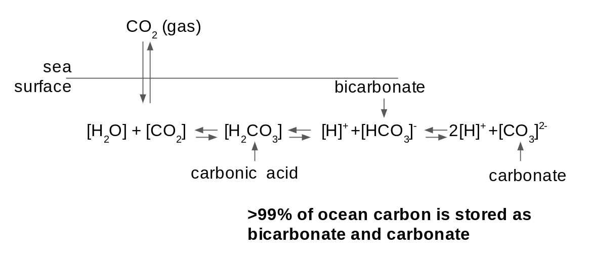
Figure 1: Chemical reactions once CO2 enters seawater
The capacity to hide CO2 in chemical species other than CO2 is buffer capacity. The additon of carbon to the surface ocean reduces buffer capcity by altering the chemistry. Ultimately less CO2 is hidden, and thus \(\delta_t pCO_{2}^{ocn}\) increases more for the same perturbation to Dissolved Inorganic Carbon (\(\delta_t DIC = C_{ant}\)) (Figure 2).
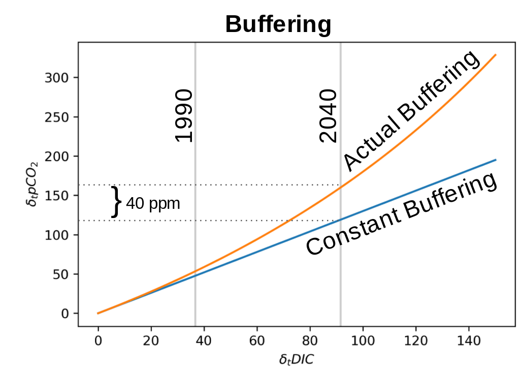
Figure 2: The vertical gray lines are mixed layer \(\delta_t DIC\) concentrations in 1990 and 2040 in the RCP8.5 scenario. The loss of buffer capacity results in \(\delta_t pCO_{2}^{ocn}\) being 40 ppm higher in 2040.
Buffer capacity can be fixed to preindustrial values in QOCCM by setting the chemistry flag to “constant”:
# linear buffering
ds = ocean_flux(atmos_co2,
                OceanMLDepth=OceanMLDepth, HILDA=True,
                DT=None,
                temperature='variable', chemistry='constant',
               )
Constant Temperature
Gases are more soluable at colder temperatures, thus as the ocean surface warms, less CO2 will be able to dissolve in the ocean surface (Figure 3). This is the dominant impact of warming associated with unmitigated climate change prior to 2080 (Ridge and McKinley 2020). Beyond 2080, effects of changing ocean circulation start to grow (Randerson et al., 2015; Ridge and McKinley 2020), which are not represented by QOCCM, so keep in mind that high warming simulations that use QOCCM beyond 2080 are missing a key mechanism of change.
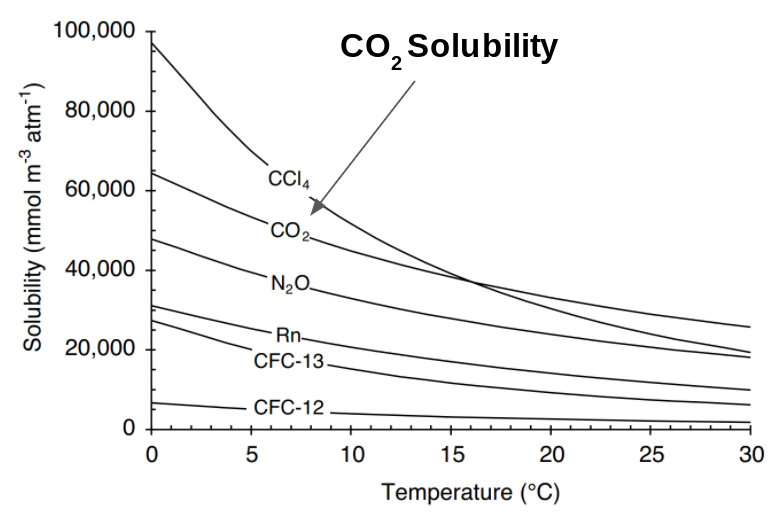
Figure 3: Gas solubility for various gases, including CO2. Figure from Sarmiento and Gruber (2006).
Solubility can be fixed to preindustrial values in QOCCM by setting the temperature flag to “constant”:
# constant temperature
ds = ocean_flux(atmos_co2,
                OceanMLDepth=OceanMLDepth, HILDA=True,
                DT=None,
                temperature='constant', chemistry='variable',
               )